What is the ROW function in Excel?
→ The MS Excel ROW function returns the ROW number of a cell reference.
→ The ROW function is a built-in function in Excel.
→ We can put this function into the Lookup/Reference Function category.
How to use the ROW function in Excel?
→ This function can be entered as part of a formula in a cell of a worksheet.
What is the return value of the ROW function?
→ The ROW function returns the numeric value of the ROW.
What is the Syntax of the ROW function?
The syntax of the ROW function in Microsoft Excel is mentioned below:
=ROW([reference])
👉 The Syntax Parameter or Syntax Arguments are:
→ Reference – It is the reference of the cell or cell range for which we need to check the ROW number
👉 Note:
→ The ROW Function returns the ROW number of a reference cell.
→ For example, =ROW(C5) returns 3 since C is the third ROW in the spreadsheet.
→ ROW takes just one argument, that argument is known as "a reference".
→ And that reference can be empty or a reference can be a single cell address or a range of cells.
→ We can say that the reference is optional
→ The reference cannot include multiple references or addresses.
→ If we will not provide any reference then the ROW returns the ROW number of the cell in which we have applied the formula.
→ No need to worry about the above notes we will understand with the help of the different examples that are mentioned below.
Examples of ROW Function
→ For better understanding of COLUMN function we will refer the below three different examples.
Example-01: ROW Function with Cell Reference
→ We will use this function to check the ROW reference number with the help of the cell number.
→ As per the syntax of the ROW Function (i.e. =ROW([reference])), we will apply this function to cell number A1 and cell number D3.
→ So this function will return the ROW number that is associated with the cells A1 and D3 that is mentioned below.
=ROW(A1)
→ The above formula will return 1. The 1 is the associate ROW number of cell A1.
=ROW(D3)
→ The above formula will return 3. The 3 is the associate ROW number of cell D3.
→ For better understanding refer to the below picture.
Example-02: ROW Function without Reference
→ We will understand the ROW Formula without any reference provided in the formula.
→ If we will not provide any reference then the ROW returns the ROW number of the cell in which we have applied the formula.
→ Let us say if we provide the formula =ROW() into cell C5 then this formula will return 3.
→ The 3 is associated with cell C3.
→ Similarly if we provide the formula =ROW() into cell D7 then this formula will return 7.
→ The 7 is associated with cell D7.
Example-03: ROW Function with Range as a Reference
→ In this example we will understand if we mention a range in formula reference then it will return the row numbers for that range.
→ For better understanding we will refer to the below formula as per the syntax =ROW(reference)
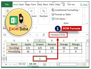
=ROW(C1:E3)
→ The above formula will return {1,2,3} and will split vertically into 3 cells.
→ So it will return the range of row numbers for the mentioned range.
→ The return value {1,2,3} is known as an array and it is only supported in the Dynamic Array Formula supported version of Excel and that is Microsoft Office 365.
→ The older version of Excel will return the value of the starting row.
→ So, the older version of Excel will return as value 1 for the above-mentioned formula =ROW(C1:E3)
→ Refer to the below photo for better understanding.
👉 For a regular update:
➨ Join us (Telegram Channel)
➨ Join us (LinkedIn Page)
👉 Also Navigate Our Popular Category:
➨ Lookup & Reference Functions


Post a Comment