What is a SUMIF function in Excel?
→ SUMIF function is used for making the sum of cells that meet a single
condition.
→ In simple language, SUMIF_function helps us to make a sum of numbers in a
defined range that meets specifically defined criteria.
→ We can use logical operators like (Greater Than (>), Less Than (<),
Not equal to something (<>), Equal to (=)), and wildcards
operator The asterisk (*) = character matches zero or more
characters, question mark(?) = character matches with
single characters for defining the criteria.
→ The criteria may be the exact match or it may be the partial match. In
both conditions, this_function will help us.
→ This function returns a numeric value.
How to use the SUMIF function in Excel?
→ You can refer to the Microsoft Excel tutorial to understand the SUMIF
function.
→ SUMIF_function explained below with examples.
→ We can simply use this function by adding the formula in the cell.
What is the syntax of the SUMIF function?
→ The syntax for the SUMIF function in Microsoft Excel is:
=SUMIF (range, criteria, [sum_range])
The Syntax Parameter or Syntax Arguments are:
➨ range ⇒ It is the range of cells from that we
need to decide and apply the criteria.
➨ criteria ⇒ It is used to determine
which cells to be added during the sum.
➨ sum_range ⇒ It is the range of cells
form that we need to make sum if the specific condition will mate. In other
words, if the criteria will fulfill then the numbers will be added from the
sum_range.
Examples of SUMIF Function in Excel:
→ For a better understanding of the SUMIF function, we can take one example.
→ In the below picture we can see the different cars sold in different
years.
→ So we need to make a sum for a specific model which model sold and what is
the sold quantity.
→ For this, we will use the SUMIF function.
Example: We need to count the total qty of BMW cars sold.
→ So from the syntax, we know that the SUMIF function has three
parameters/arguments. We will understand one by one with the help of the
Excel formula
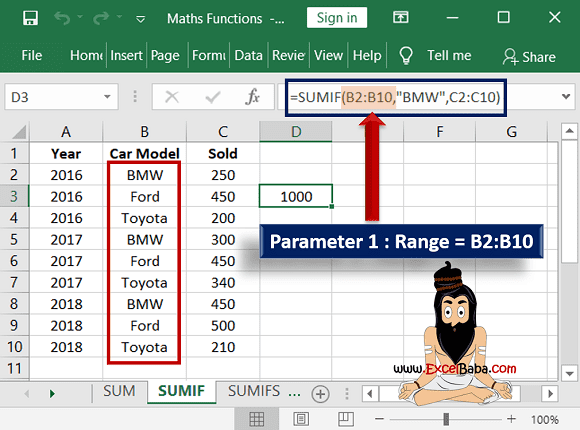
➨ Parameter 1: Range
→ The first parameter in the SUMIF function is the “range”. So we need to
decide from which range we need to compare the criteria.
→ In our case, we need to check the sold qty of the BMW car. So our criteria
is “BMW”. BMW is available in the cell_range B2:B10.
→ So our Range = B2:B10 in this example.
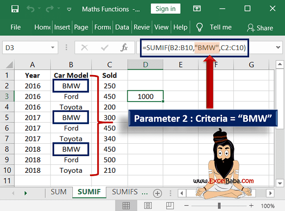
➨ Parameter 2: Criteria
→ In simple words from the selected range of for which product/category we
want to make sum is called the criteria.
→ In the above example, we need the sum of BMW car sold from the selected
range so our category is “BMW”. (Note: If we are mentioning the criteria as
a text then we need to add text in between the double invited comma “”. E.g.
“BMW”).
→ We can mention criteria with two different methods. (1) we can mention as
“BMW” or (2) We can give reference of cell-like in the above example we can
give the cell reference = B2 cell because the value of B2 cell is BMW.
➨ Parameter 3: Sum Range
→ The third parameter of the SUMIF function is the range of numbers that
will be added together.
→ In other words, in our example, we need to make sum of sold qty of BMW car
and sold qty is available in cell_range C2:C10. So this is our sum_range.
→ From this range, the sum will be made.
→ So as mentioned in above example we have applied the formula
=SUMIF(B2:B10,"BMW",C2:C10).
→ This formula find the car name "BMW" from the range B2:B20 and make sum
from sum_range C2:C10.
→ So we can get the result as total BMW car sold = 1000.
👉 For a regular update:
➨ Join us (Telegram Channel)
➨ Join us (LinkedIn Page)
👉 Also Navigate Our Popular Category:
➨ Lookup & Reference Functions


Post a Comment