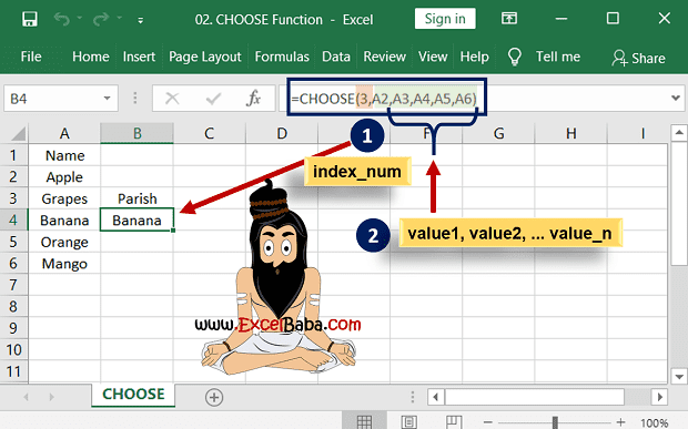
What is the CHOOSE function in Excel?
→ The CHOOSE function returns a value from the list of a given position or index value.
→ The value may be any of a number, a cell reference, a defined name, a formula/function, or a text value.
→ It is a built-in function in Excel and we can put it in the Lookup or Reference Function category.
→ It can be used as a worksheet function in Excel. So we can enter this function directly into the cell.
What is the syntax of the CHOOSE function?
→ The syntax for the VLOOKUP function in Microsoft Excel is:
=CHOOSE(index_num, value1,[value2, ... value_n])
The Syntax Parameter or Syntax Arguments of CHOOSE function are:
➨ index_num - The position in the list of values to return. It must be a number between 1 and 29.
➨ value1, value2, ... value_n - A list of up to 29 values. A value can be any one of the following: a number, a cell reference, a defined name, a formula/function, or a text value.
Important Points for using CHOOSE function
→ The CHOOSE function returns any datatype such as a string, numeric, date, etc.
→ If we mentioned the position is less than 1 in index_num then the CHOOSE function will return error #VALUE!.
→ If we mention the position is greater than the number of values in the list, the CHOOSE function will return the error #VALUE!.
Examples of CHOOSE Function:
→ We will learn two different examples for understanding the CHOOSE Function
Example 1: CHOOSE function with Defined Name
→ As we know the syntax of CHOOSE function =CHOOSE(index_num, value1,[value2, ... value_n])
→ So we are mentioned the different city’s name and pull out the value from the formula.
→ As we can see in the below picture that the formula =CHOOSE(3,"New York","Washington","Parish","Dubai").
→ It will return the result=Parish. Because the Parish is in the 3rd position from the value list.
Example 2: CHOOSE function with cell refrence
→ As we know the syntax of CHOOSE function =CHOOSE(index_num, value1,[value2, ... value_n])
→ In this example, we will mention the cell reference from the Excel worksheet.
→ The formula will be =CHOOSE(3,A2,A3,A4,A5,A6)
→ So the above formula will return the 3rd value from the value list.
→ That will be the value available in the cell no A4.
→ We will get the result =Banana.
👉 For a regular update:
➨ Join us (Telegram Channel)
➨ Join us (LinkedIn Page)
👉 Also Navigate Our Popular Category:
➨ Lookup & Reference Functions


Post a Comment