What is the SUMIFS function in Excel?
→ The Microsoft Excel SUMIFS function adds all numbers in a range of cells, based on single or multiple criteria.
→ In simple language, the SUMIFS function helps us to make sum of all numbers that fulfill the single or multiple conditions.
→ The criteria may be the exact match or it may be the partial match.
→ In both conditions, this function will help us. This function supports the logical operators (>,<,<>,=) and wildcards (*,?) for partial matching.
→ The SUMIFS function returns a numeric value.
➨ How to use the SUMIFS function in Excel?
→ Refer to this article for the SUMIFS function explained with examples. We need to enter a simple formula in MS Excel spreadsheets for making the sum of single or multiple conditions fulfill.
What is the syntax of the SUMIFS function?
→ The syntax for the SUMIFS function in Microsoft Excel is:
=SUMIFS(sum_range, criteria_range1, criteria1, [criteria_range2, criteria2, ... criteria_range_n, criteria_n])
➨ The Syntax Parameter or Syntax Arguments are:
→ sum_range – This is the cell range from which we want the sum.
→ criteria_range1 - The range of cells that you want to apply criteria1 against.
→ criteria1 - It is used to determine which cells to add. criteria1 is applied against criteria_range1.
→ criteria_range2 ... criteria_range_n – This is an optional command if we want to add more than one criterion then it will be used. It is the range of cells that you want to apply criteria2 ... criteria_n against the criteria_range. We can add up to 127 ranges.
→ criteria2, ... criteria_n – This is an optional command. It is used to determine which cells to add. criteria2 is applied against criteria_range2, criteria3 is applied against criteria_range3, and so on. We can add to 127 criteria.
Examples of SUMIFS Function:
→ For a better understanding of the SUMIFS function, we can take one example.
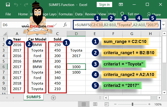
→ In the below picture, we can see the different cars sold in different years.
→ So we want how many Toyota cars were sold in 2017.
→ In this example, we have multiple criteria for comparison so we will use the SUMIFS function.
→ Example: We need to count the qty of Toyota Car sold in the year 2017.
→ So, from the syntax, we will use the below formula for the making sum of the total Toyota car sold in the year 2017.
=SUMIFS(C2:C10,B2:B10,"Toyota",A2:A10,"2017")
➨ From the above formula,
- sum_range = C2:C10 (Make sum of car qty sold.)
- criteria_range1 = B2:B10 (Check criteria1 “Toyota” from this range.)
- criteria1 = “Toyota”
- criteria_range2 = A2:A10 – (Check criteria2 “2017” from this range.)
- criteria2 = “2017”
→ Also, we can use cell reference instead of the criteria’s absolute value in the above formula as mentioned in the below formula.
=SUMIFS(C2:C10,B2:B10,D3,A2:A10,D4)
→ So we have used cell reference (D3) instead of absolute value (Toyota) and used to mention D4 instead of "2017" in the above example.
👉 For a regular update:
➨ Join us (Telegram Channel)
➨ Join us (LinkedIn Page)
👉 Also Navigate Our Popular Category:
➨ Lookup & Reference Functions


Post a Comment